Direct ɣ in d+Au collisions
The measurement of γ and π0 yields in d+Au interactions is important for studying the formation of quark-gluon plasma (QGP) in heavy ion collisions.
One way to measure QGP formation is by observing jet suppression using the nuclear modification factor RAB, which compares the yield of a particle (in this case, the π0) in AB collisions to that in p+p collisions. RAB is calculated by dividing the invariant yield measured in AB collisions by Ncoll times the invariant yield measured in p+p collisions. If RAB is equal to one, then the yield observed in AB is the same as that observed in p+p. If RAB is less than one, then the yield in AB is suppressed, and if it is greater than one, then it is enhanced.
For a more detailed explanation that includes the motivation and physics
background, please refer to this write-up:
![]() .
.
- Direct ɣ in d+Au collisions
- The Analysis Outline
- General Analysis Workflow Diagram
- Source Code
- Input Data
- Calibration Dependencies
- Running the Analysis in Containers
- Running the Analysis with REANA
- Confirming the Results
- Analysis Steps
- 1a. Raw π0 spectrum (MB + ERT)
- 2a. π0 simulation
- 3a. 2D response matrix of π0 momentum reconstruction
- 5. Corrected π0 spectrum
- 6. Corrected η spectrum
- 7. Decay γ spectrum from π0
- 8. Decay γ spectrum from η, η’, and Ω
- 9. Total decay γ spectrum from π0, η, η’, and Ω
- 10. Modified inclusive γ spectrum
- 11. Raw direct γ spectrum
- 12. Corrected direct γ spectrum
- 13. Direct γ invariant yield
- 14. π0 invariant yield
- The Analysis Outline
The Analysis Outline
This analysis was performed by Dr. Niveditha Ramasubramanian. The goal of this page is to consolidate information in a way that is sufficient to make reproduction of the analysis possible.
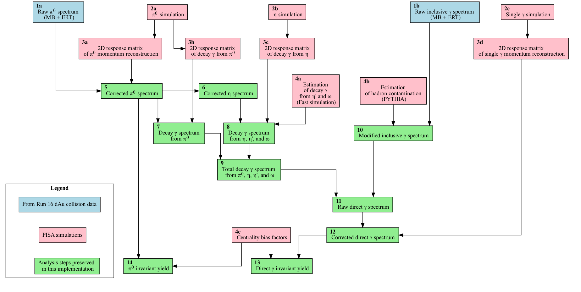
General Analysis Workflow Diagram
Source Code
The code prepared for preservation can be found in the ana-dAuPi0Photon repository
on the gitea server maintained by the BNL SDCC, accessible to PHENIX members with BNL
credentials:
https://git.racf.bnl.gov/gitea/PHENIX/ana-dAuPi0Photon
The original location of the analisys code and supplementary files is in
/gpfs/mnt/gpfs02/phenix/plhf/plhf1/nivram/ accessible from the BNL SDCC’s
interactive nodes.
Input Data
Parts of this analysis use data samples kept in the storage area intended for long-term preservation. This is its location in the GPFS filesystem of BNL SDCC:
/gpfs/mnt/gpfs02/phenix/data_preservation/phnxreco/emcal
Additional input files are stored in the Zenodo repository
![]()
Calibration Dependencies
There are “DeadWarn” and “Timing” type of maps which are prerequisite of this
analysis and they are considered as a separate “prior” component. In a condensed
form, they are preserved in the folder sim_Pi0Histogram in the gitea repository mentioned above.
Running the Analysis in Containers
In order to run the analysis steps preserved in this implementation, i.e. the
blue and green boxes shown on this
flowchart,
one can use either singularity or docker.
Singularity
mkdir output_plots
singularity run -B $PWD/output_plots:/dAuPi0Photon/output_plots docker://registry.sdcc.bnl.gov/dap-phenix/dauphotonpi0
Docker
docker run -v $PWD/output_plots:/dAuPi0Photon/output_plots registry.sdcc.bnl.gov/dap-phenix/dauphotonpi0
Building the Image
If any of the files change in the analysis repository, the following commands can be used to rebuild the image and push it to the registry:
cd ana-dAuPi0Photon
docker build -t registry.sdcc.bnl.gov/dap-phenix/dauphotonpi0 .
docker push registry.sdcc.bnl.gov/dap-phenix/dauphotonpi0
Running the Analysis with REANA
Each step of the analysis can be executed by using the corresponding workflow
defined in the YAML files. For example, to run the code in block N, issue the
following command in the terminal:
reana-client run -f N_reana.yaml -w N_reana
The input files will start uploading to the server, and you can check the job
status by pointing your browser to $REANA_SERVER_URL. Once the job is
complete, you can use the reana-client commands to list the files in the
workspace’s working directory on the server and download the output results to
your local machine.
To list the files in the workspace’s working directory on the server, use the following command:
reana-client ls -w N_reana
To download the output results to your local machine, use the following command:
reana-client download -w N_reana path/to/output/file.dat
To select a specific set of files, you can combine the above commands using Linux piping, for instance:
reana-client ls -w N_reana | grep output_plots/txt/ | cut -d' ' -f1 | xargs reana-client download -w N_reana
Confirming the Results
One can verify that the output produced is identical to the reference saved in the repository. The following command should return no differences in the output files:
git clone https://github.com/PhenixCollaboration/ana-dAuPi0Photon.git
cd ana-dAuPi0Photon
diff -r path/to/output_plots/txt output_plots_ref/txt
Analysis Steps
Finally, we provide further details below for each of the analysis steps referenced by their “block numbers” defined in the analysis workflow diagram.
1a. Raw π0 spectrum (MB + ERT)
The analysis starts with files produced by the Taxi process. The ROOT macro pi0Extraction.cc takes the Taxi ROOT files as input and generates MB (min bias)
and ERT (triggered) data as output. This macro is included in a driver script corrPi0Chain.csh.
# condor_Pi0Extraction.cc reformatted and renamed "pi0extraction.C"
root -l -b -q 'pi0extraction.C("MB", "PbSc", 4,5)'
root -l -b -q 'pi0extraction.C("ERT", "PbSc", 4,5)'
root -l -b -q 'WGRatio.C' # Merging MV and ERT spectra of raw pi0 with normalization

# The outputs of this step are placed in the output_plots folder,
# in three subfolders pdf, root, txt
These commands are included in pi0extraction.yaml.
Currently a folder output_plots is created with subfolders txt,root,pdf,
and the folder txt contains the actual analsys data.
2a. π0 simulation
Presented below is the core of this workflow which includes processing of multiple input files (60 in total):
# the original code found in the Condor submission part:
root -l -b <<EOF
  .L Pi0EmbedFiles.C
   Pi0EmbedFiles t
   t.Loop()
   EOF
Adaptation of the ROOT macro for REANA, in a separate file pi0run.script:
gSystem->Load("libTHmul.so");
.L Pi0EmbedFiles.C
Pi0EmbedFiles t
t.Loop()
In the REANA script, this is used as follows: cat pi0run.script | root -b.
Note that a PHENIX-specific ROOT library libTHmul.so is loaded
in the beginning, as this is necessary for proper operation of the macro.
Please refer to the relevant folder in the PHENIX GitHub repository for access to the actual material.
This is the driver script Pi0EmbedFiles.csh. Note that symbolic links are created
to feed successive files from a holding folder, to the ROOT macro.
#!/bin/tcsh
source ./setup_env.csh

foreach i (`seq 0 1 $1`)
    ln -s gpfs/mnt/gpfs02/phenix/data_preservation/phnxreco/emcal/Pi0/test/simPi0_$i.root pi0_dAuMB.root
    echo File: $i
    ls -l pi0_dAuMB.root
    cat pi0run.script | root -b
    mv EmbedPi0dAu.root EmbedPi0dAu_$i.root
    rm pi0_dAuMB.root
end
tar -cf embedPi0dAu.tar EmbedPi0dAu_*
Processing of input files takes place sequentially and in this case takes a significant amount of time compared to other steps, i.e. a feew hours.
The results of all emedding runs are bundled together in a tar archive to make downloading easier. Upon
retrieval the data need to be merged using the utility haddPhenix which is done in block 3a (see below).
Upon completion of this step the file embedPi0dAu.tar needs to be downloaded, and put
in the folder from where the next step is launched. An example of the cownload command, assuming the workflow
was named “embed”:
reana-client download -w embed embedPi0dAu.tar
3a. 2D response matrix of π0 momentum reconstruction
In this step we call a function in ROOT macro generationRM_Pi0.C that creates a set of ROOT
histograms. The histograms represent the response matrix (RM) for the π0 meson
production in heavy-ion collisions. The function reads an input ROOT file named EmbedPi0dAu.root
and creates a new output ROOT file named Pion_RM.root. The function calculates the RM by
dividing the Pt response (pTecore vs. generated Pt) for different centrality bins, particle
identification (PID), and detector sectors. The RM is stored in a 2D histogram (TH2D) with Pt bins.
The output response matrix represents the probability for a π0 particle with a given
generated momentum to be measured with a different momentum due to detector effects.
Tar file containing multiple ROOT files (see previous step 2a) is uploaded as input for this step.
Abbreviated contents of driver script look as follows:
#!/bin/tcsh
source ./setup_env.csh
haddPhenix EmbedPi0dAu.root EmbedPi0dAu_*
root -l -b -q 'generationRM_Pi0.C'
The macro generates the file EmbedPi0dAu.root by merging inputs via haddPhenix
and produces Pion_RM.root. The complete description is in generationRM_Pi0.yaml,
which resides with all subsidiary scripts in the folder generationRM.
The workflow description is as follows:
version: 0.0.1
inputs:
  files:
    - ./setup_env.csh
    - ./generationRM_Pi0.C
    - ./generationRM_Pi0.csh
    - ./embedPi0dAu.tar
workflow:
  type: serial
  specification:
    steps:
      - environment: 'registry.sdcc.bnl.gov/sdcc-fabric/rhic_sl7_ext:1.3'
        commands:
        - tar xvf embedPi0dAu.tar
        - chmod +x ./generationRM_Pi0.csh
        - ./generationRM_Pi0.csh > output.txt
        - ls -l >> output.txt

outputs:
  files:
    - output.txt
    - Pion_RM.root
The result will need to be downloaded as follows (assuming the worflow was assigned the name “gen” in REANA - can be anything):
reana-client download -w gen Pion_RM.root
5. Corrected π0 spectrum
This REANA step (final in this analysis)
is accomplished with scripts and macros named VConvolution_Pi0*. The file Pion_RM.root
serves as input, along with text files residing in output_plots previosly produced by the macros
pi0extraction.C and WGRatio.C:
scaledUEB_rawPi0_ERT_PbSc_0CC88_Chi2_3Sig.txt
scaledUEB_rawPi0_MB_PbSc_0CC88_Chi2_3Sig.txt
scaledUEB_rawPi0_BBCpERT_PbSc_0CC88_Chi2_3Sig.txt
The core of this step looks like this:
root -l -b -q 'VConvolution_Pi0.C'
The REANA submission file has this content:
version: 0.0.1
inputs:
  directories:
    - ./output_plots
  files:
    - ./inputTrialFunction_Pi0.txt
    - ./setup_env.csh
    - ./VConvolution_Pi0.C
    - ./VConvolution_Pi0.csh
    - ./Pion_RM.root
workflow:
  type: serial
  specification:
    steps:
      - environment: 'registry.sdcc.bnl.gov/sdcc-fabric/rhic_sl7_ext:1.3'
        commands:
        - chmod +x ./VConvolution_Pi0.csh
        - ls -l > output.txt
        - ./VConvolution_Pi0.csh >> output.txt
        - ls -l >> output.txt

outputs:
  files:
    - output.txt0
Outputs are also written in output_plots/txt and contain
scaledEB_corrPi0_BBCpERT_PbSc_0CC88_Chi2_3Sig.txt
scaledUEB_corrPi0_BBCpERT_PbSc_0CC88_Chi2_3Sig.txt
6. Corrected η spectrum
This step is implemented using two functions getEtaSpectrum and
getEtaSpectrum_UEB that process data from the input files and applies
correction factors to obtain the spectrum of eta particles in different
centrality bins.
Inputs:
scaledEB_corrPi0_BBCpERT_
scaledUEB_corrPi0_BBCpERT_
Outputs:
scaledEB_corrEta_BBCpERT_
scaledUEB_corrEta_BBCpERT_
7. Decay γ spectrum from π0
In this, we take the corrected pion spectrum from the convoulution procedure and
then multiply it by the gamma response matrix and obtain the decay gamma
spectrum for pions. See VconvolutionRMgamma_Pi0.
Inputs:
scaledEB_corrPi0_BBCpERT_
scaledUEB_corrPi0_BBCpERT_
rawDG_Pion.root
Outputs:
scaledUEB_rawDGPi0_BBCpERT_
8. Decay γ spectrum from η, η’, and Ω
In this we take the corrected pion spectrum from the convoulution procedure and
then multiply it by the gamma response matrix and obtain the decay gamma
spectrum for pions. See VconvolutionRMgamma_Eta.
Inputs:
rawDG_Eta.root
scaledEB_corrEta_BBCpERT_
scaledUEB_corrEta_BBCpERT_
Outputs:
scaledUEB_rawDGEta_BBCpERT_
withTimingDM_1p4Sig_VconRMgamma.root
9. Total decay γ spectrum from π0, η, η’, and Ω
rawDG_EPP
Inputs:
scaledUEB_rawDGEta_BBCpERT_
scaledUEB_rawDGPi0_BBCpERT_
Outputs:
scaledUEB_rawDGEPP_BBCpERT_
10. Modified inclusive γ spectrum
getNewSpectrum
Inputs:
landauEval.txt
scaledUEB_rawIP_BBCpERT_
Outputs:
scaledUEB_newrawIP_BBCpERT_
11. Raw direct γ spectrum
rawDP
Inputs:
scaledUEB_rawDGEPP_BBCpERT_
scaledUEB_newrawIP_BBCpERT_
Outputs:
scaledUEB_rawDP_BBCpERT_
12. Corrected direct γ spectrum
VconvolutionRM_Photon
Inputs:
AN1371_spectrumPoints.txt
Photon_RM.root
scaledUEB_rawDP_BBCpERT_
Outputs:
scaledEB_corrDP_BBCpERT_
scaledUEB_corrDP_BBCpERT_
13. Direct γ invariant yield
Centrality_corrDP_highPt
Inputs:
statErr_corrDP_BBCpERT_
Outputs:
invyield_corrDP_BBCpERT_
14. π0 invariant yield
Centrality_corrPi0_highPt
Inputs:
statErr_corrPi0_BBCpERT_
Outputs:
invyield_corrPi0_BBCpERT_