Pad Chamber hit reconstructionThis document describes the Pad Chamber hit reconstruction algorithms as well as performance. By Paul Nilsson, Lund University 1. PreliminariesWhat is a pad anyway? And what about pixels and cells? Let us start with the chamber itself. In the PHENIX experiment there are three thin layers of pad chambers (called PC1-3) in one of the two central arms, and two layers in the other (PC1,3) providing three-dimensional coordinates along the charged particle trajectories in the field-free region (see Fig. 1).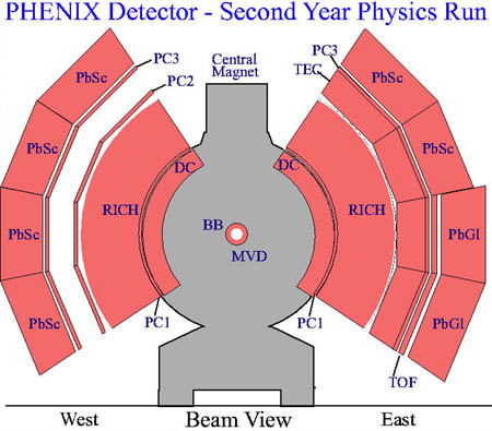 Fig 1. The central arms in the PHENIX experiment. A pad chamber is a wire chamber equipped with pad readout. A wire chamber is usually read out on the wires. However, when the multiplicity gets high this will inevitably lead to ambiguities that are hard to compensate for. By placing a pad plane directly behind the wire plane, positive ions caused by avalanches in the gas will be sensed on the pads, while the wires will pick up the avalanches. The pad plane solves the wire ambiguity problem since it is divided into many small copper electrodes, called pads, that are read out individually giving two dimensional hit information. The position of the chamber gives the third coordinate. Fig 2. The area formed by the three outlined pixels in the center [right], each belonging to a different but adjacent pad [left], constitute a cell. Numbers are for PC1. A PHENIX pad consists of nine smaller connected rectangles called pixels (see Fig. 2). By arranging the pads in a repeated interleaved pattern, a factor of three in the number of readout channels can be saved with marginal loss of performance. The area formed by three pixels belonging to three different but adjacent overlapping pads is called a cell (see Fig. 2). Details about PC geometry and numbering conventions can be found in separate documents (http://www.kosufy.lu.se/phenix/convention.shtml). 2. Pad Chamber reconstructionThe response of the pad chambers is simulated within the PHENIX software framework. The event generator HIJING1.35 is used to feed PISA (i.e. GEANT) with events. The PISA output containing the hit information, is then used as input for the reconstruction code.2.1 An object oriented approachBrowsified code can be found athttp://www.phenix.bnl.gov/phenix/WWW/publish/nilsson/tech/html/ neither of which might be the latest version. The Pad Chamber reconstruction objects, with pointer names Pc1Rec, Pc2Rec and Pc3Rec, are
instances of the PadRecModule class and are created in the preco
code, padfuncs.C. The object initializations are also done
here (such as cluster splitting on/off, which geometry database to read from
(ASCII/Objectivity), cluster sizes and other limits). The main hit
reconstruction algorithm is located in the event method of the
PadRecModule class. This instantiates an object from the
PadRec class needed for the reconstruction, with pointer name
padRecObj. This class contains all of the methods applied to the
padRecObj objects in the main reconstruction algorithm. The
decision to have two classes instead of one was made at a time when root had
poor support for the standard template library (STL). It was necessary to
avoid STL usage in code to be used in root dictionary generation. The STL is of
fundamental importance in the code since cell clusters are easily built and
maintained using the STL list objects. Finally, the
PadRecCell class are used to define the cell objects
stored in the STL lists.
2.2 The response simulatorThe PISA hit information is processed with a response simulator (when running with simulated data). For each track, the deposition of charge on the chamber wires is estimated using a Landau distribution with the addition of random electronics noise. The output is a list of all pads that have received charge above a certain threshold.2.3 The cluster reconstruction algorithmThe cluster reconstruction code reads the list of fired pads and translates it into a list of cells, which is more easy to work with. The outline of the main algorithm (Fig. 3) is to first identify a group of one or more cells, called a cluster, and then process each cluster separately to determine the original hit position. The used cells are removed from the list. The number of particles that have created the cluster is estimated by analyzing the cluster size. If the number is larger than one, the cluster is split into subclusters according to size and symmetry arguments (see section 2.3 below). The last step of the algorithm calculates the center of each subcluster and transforms it from cell space into the global PHENIX coordinate system.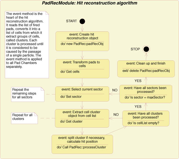 Fig 3. Diagram showing the program flow of the PC cluster reconstruction algorithm. The stored hit information is used in the track finding and the momentum reconstruction. When possible, the DC uses the PC1 z-coordinates to define the tracks. 2.4 Cluster splittingWhen two or more charged particles pass through a chamber at close distance from each other, charge is deposited on many pads resulting in a large cluster of several cells. In order not to loose resolution in the Pad Chambers, these large clusters need to be split until each sub cluster is considered to be caused by a single charged particle. This is deemed to be the case if the cluster fit inside a square covering 4x4 cells with a maximum of 11 fired cells.Fig. 4 describes in detail how the split algorithm works. Using the cluster split algorithm recovers about 34% of the hits that otherwise will be lost due to cluster overlap. 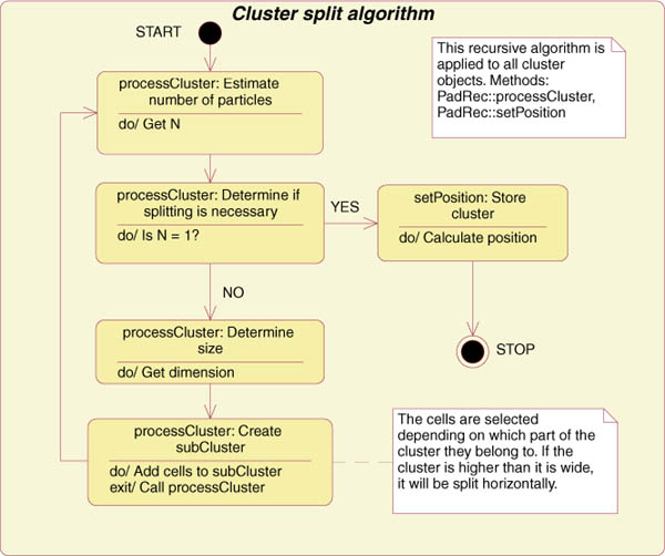 Fig 4. If a cluster is considered to be caused by the close passage of two or more tracks, it will be split until each subclusters is a single-particle cluster. The diagram shows the program flow of the recursive split algorithm. The plots in the following sections for simulated data were all generated with cluster splitting turned on. With real data the picture is more complicated due to large clusters created by single particles entering sideways in the chamber, long range delta electrons, slow moving highly ionizing protons, sparks, etc. These effects are subject to continued studies. 3. Cell multiplicity distributionsThe threshold settings in the response simulator have been tuned by comparing single particle cluster sizes from cosmics with the corresponding clusters in simulated data.A comparison between data and simulation can be seen in Fig. 5 for PC3 (PC1 looks the same while data from PC2 were not available at the time of the study). The cell multiplicity, i.e. the number of cells per cluster, is stored in the type variable in the dPadCluster
table. A negative type value means that the cluster was split
(i.e. the cluster is in fact a sub-cluster coming from a split cluster). This
investigation should also be done for PC2 (later). The threshold setting for
PC2 in the simulation is an interpolation of the PC1 and PC3 values.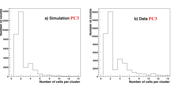 Fig 5. Cell multiplicity distributions for PC3 from simulation and data (produced with cluster splitting turned ON). As can be seen from the above pictures, the agreement is good between data and simulation in terms of 1 to 2 cell clusters. There are bigger clusters present in data due to physical effects not present in the simulation as mentioned above (section 2.4). 4. Position resolutionThe position resolution was determined by comparing the reconstructed hit positions were compared to the true hit positions according todz = zREC - zPISA where y is the coordinate across the wires and z is the coordinate along the wires, which is also along the beam direction. The position resolutions were also experimentally estimated using cosmics. The details of this study can be found in the long PC NIM paper. Fig. 6-8 shows the simulated position resolutions for PC1-3 respectively, while table 1 summarizes the position resolutions from both simulation and measurements. 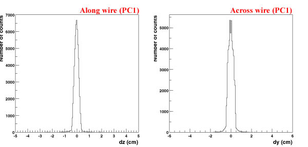 Fig 6. a) The position resolution along the wire for PC1 (in cm). b) The position resolution across the wire for PC1 (in cm).  Fig 7. a) The position resolution along the wire for PC2 (in cm). b) The position resolution across the wire for PC2 (in degrees). 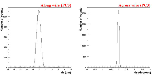 Fig 8. a) The position resolution along the wire for PC3 (in cm). b) The position resolution across the wire for PC3 (in degrees). Note that the resolution across the wire for PC2/3 are given in degrees in the plots (by mistake).
The measured values are from the cosmics measurements described in the long NIM PC paper. The position resolution in PC3 was not measured. 5. Two-track resolutionBy simulating minimum ionizing pi+ pairs with small separation in PISA, the probability for resolving nearby tracks was calculated. The momenta of the pions were chosen as the rule of thumb value of 500 MeV. A more careful calculation gives that the momentum of a minimum ionizing pion is about 460 MeV with beta = 0.957. The two-track resolution is in this context defined as the distance where 50% of the tracks are separated. Shown in Fig. 9-11 are the two-track resolutions along and across the wires for PC1-3. Numbers are given in Table 2.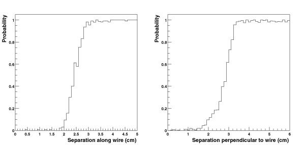 Fig 9. a) The two-track resolution along the wire for PC1. b) The two-track resolution across the wire for PC1. 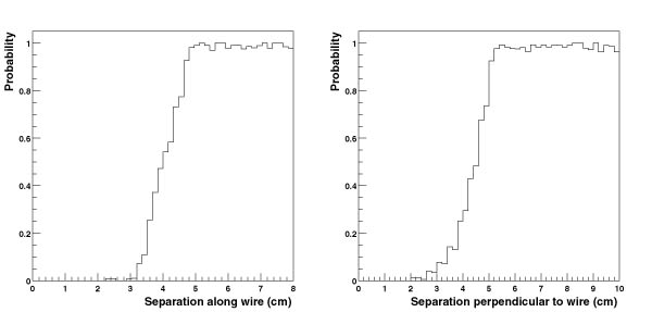 Fig 10. a) The two-track resolution along the wire for PC2. b) The two-track resolution across the wire for PC2.  Fig 11. a) The two-track resolution along the wire for PC3. b) The two-track resolution across the wire for PC3.
6. Reconstruction efficiencyDue to severe bugs in the PC response simulator (sometimes pads don't fire although charge greater than the threshold value is deposited in PISA), the reconstruction efficiency cannot be directly calculated from simulation. Real data was therefore used to calculate the reconstruction efficiency for PC1. Drift chamber tracks with a quality factor of at least 3 (X1+X2) were projected in the XY-plane to PC1. The closest PC1 hit was determined. To keep ambiguities in the z-direction to a minimum, only peripheral collisions were used. The found PC1 reconstruction efficiency was better than 98% (consistent with J. Jia's earlier investigation). The number of ghosts has not yet been calculated. |